|
Jan-Feb 1963 event |
|
The late January-early February 1963 rainfall event produced the third largest gridpoint total. The event produced severe flooding along the Carson River Basin with a number of gage reports suggesting the flooding was 25-50 year event (FEMA). The event ranked as one of the 9 biggest floods since 1909 on the the American, Feather and Cosumnes River Basins(Roos 2007).
The strong atmospheric river associated with the California flooding also helped produce severe flooding along the Clearwater, Boise, Payette, Weiser, Portnuef and Snake River basins. Eight Idaho counties were included in a federal disaster declaration. |
|
The synoptic pattern is again very similar to the pattern of three preceding events. Each has strong positive anomaly in the vicinity of Alaska and the Bering Sea at 500-hPa with a negative height anomaly to its south with a long southwesterly fetch (see below). The combination produces a strong geopotential height gradient across northern California. A anomalous plume of moisture also extends from the sub-tropics northeastward into California indicating a strong atmospheric river is present. |
|
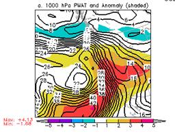
Within the atmospheric river, normalized anomalies of precipitable water exceeded 4 standard deviations (henceforth 4 sigma) just off the California coast by early Jan 31 with the PW anomaly building to over 5 sigma by 0000 UTC 1 Feb. The greater than 5-sigma PW anomaly (moisture within the atmospheric river) has a return frequency of 120 months arguing that the moisture plume associated with this system was extremely anomalous (see expected frequency figure below). . The normalized moisture flux anomalies were even higher. The greater than 5 sigma anomaly extending northward towards Idaho helps explain their severe flooding in that state. |
|
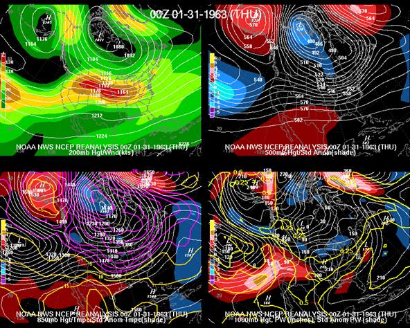
Large area 4-panel chart, 200-hPa heights and isotachs (top left), 500-hPa heights and normalized height anomaly (top right), 850-hPa heights and normalized temperature anomaly (bottom left), and 1000-hPa height and normalized PW anomaly (bottom right) valid 0000 UTC 01 Jan. 1963. The magnitude of the normalized anomalies are given by the color fill with the scale on the left had side of each panel. |
|
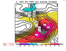
PW (mm) and normalized PW anomaly (magnitude of the anomaly scale is shown on the scale at the bottom of the figure) valid 0000 UTC 31 Jan. 1963 (top panel), 0000 UTC 01 Feb. 1963 (bottom panel). |
|
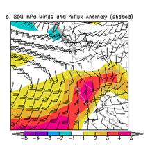
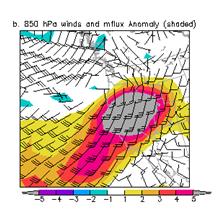
850-hPa winds (standard barbs and flags) and normalized anomaly of 850-hPa moisture flux (magnitude is given by the color fill from the bar at the bottom of the figure) valid 0000 UTC 31 Jan. 1963 (top panel), 0000 UTC 01 Feb. 1963 (bottom panel). |
|
Expected return frequency as a function of PW at a point just upstream from the Sierra Nevada mountains. X-axis is the magnitude of the normalized anomaly, the y-axis is the return frequency in months. The dotted lines highlight the return frequency of a normalized anomaly with a magnitude of 4 and shows the expected return period of 24 months. |
|
Note the rarity of having a greater than 5 sigma PW anomaly (see below). When such a high PW anomaly is present, the chances of an extreme event rises . A highly anomalous forecast of a normalized anomaly on an ensemble mean suggests the model is in strong agreement and that it is signally a pretty rare in magnitude moisture plume. |
|
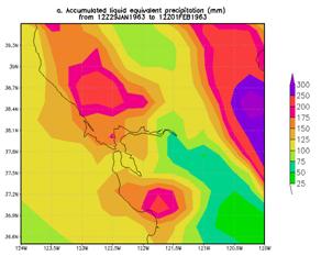
Heaviest 3-day rainfall analysis using the CDC .25 deg by .25 deg unified data set ending 1200 UCT 29 Jan 1963-1200 UTC 01 Feb 1963. |
|
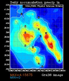
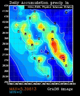
Precipitation analysis during the 24 hours (in inches) ending at 1200 UTC 30 Jan 1963 from the .25 by 2.5 deg. unified data set. |
|
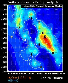
Precipitation analysis during the 24 hours (in inches) ending at 1200 UTC 31 Jan 1963 from the .25 by 2.5 deg. unified data set. |
|
Precipitation analysis during the 24 hours (in inches) ending at 1200 UTC 01 Feb 1963 from the .25 by 2.5 deg. unified data set. |