|
Exercise 1: Forecasting convective movement
|
|
In this exercise you’ll be asked to predict where a convective system is likely to develop and then predict the speed and direction in which it is most likely to move. The exercise is meant to help forecasters learn clues that might aid them in forecasting what type of MCS is most likely and help decide which vector method will most likely provide the best guess at where the MCS will track.
|
|
From the 2100 and 0000 UTC observed and forecast maps, try to determine where you think the front is located and note any differences in the pressure and low level convergence patterns that might have an impact on where convection might develop. |
|
Do you notice any areas where convergence might differ. Think why any difference might be important? |
|
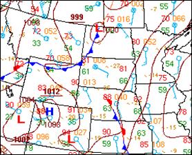
0000 UTC HPC surface map
|
|
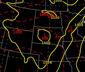
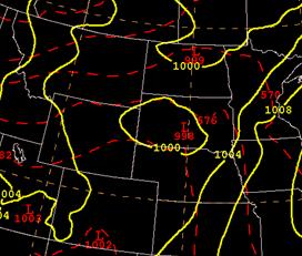
NAM MSLP forecast valid at 0000 UTC
|
|
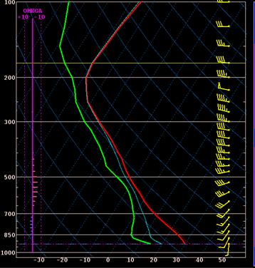
Forecast sounding valid 2100 UTC at the blue dot
|
|
The observed surface pressure pattern and wind fields at 2100 and 0000 UTC suggest that the pattern of low-level moisture convergence forecast by the NAM might be in error. For example, the observed wind field suggests low-level convergence is taking place along the front in northeastern Wyoming. |
|
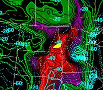
NAM CAPE and CIN forecast V.T. 2100 UTC
|
|
2100 UTC forecast sounding at the location of the blue dot in southeast SD on the earlier maps. A few important details about the sounding: CAPE=4367 J/kg, PW=1.16”, LCL=801mb, Mean RH=35%, Mean LRH=51% |
|
Using the sounding on the left (blue dot location), If you were trying to determine the mean winds of the cloud bearing layer, what layer would probably be the smartest to use?
The relatively low RH suggests that there will be decent cold pool generation by any convection that develops. There also is good potential for the downward transport of momentum to bring some of the stronger winds at mid levels down to the surface. |
|
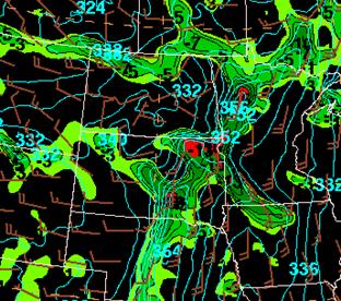
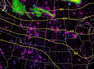
NAM 500 height and vorticity forecast V.T. 21Z
|

|
At 2100 UTC the model is forecasting one vorticity max over the central portion of the Dakotas, another over northern Wyoming and third, much stronger shortwave, extending from southern Canada southward into northern Idaho (see figures below). Based on the forecast cape, vorticity, and boundary layer convergence where would you expect convection to form within the next 3 hours? Will it be in southern South Dakota, eastern Wyoming or eastern Montana? Where the initial convection forms is important in determining the archtype of MCS that you are likely to be dealing with.
One of the big problems in forecasting the evolution and movement of an MCS is trying to predict where convective initiation will occur. The models often have problems predicting stability and can make mistakes in their predictions of the low level convergence, especially in the warm season. |
|
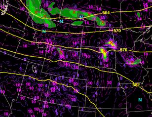
NAM 500 height and vorticity forecast V.T. 00Z
|
|
Observed 500 mb heights V.T. 00Z
|
|
Click on the radar imagery and compare the radar features shown on the loop to the evolution of the NAM forecasts of vorticity between 21Z and 00Z. Does the vorticity look real? Note that the radar echoes are decreasing as the convection moves into the region where the NAM is showing the strongest low level convergence and instability. The convection in southeastern Montana is moving eastward and looks like it may still be increasing. Your next task will be to decide which vector method you think would work best for different areas of convection. |
|
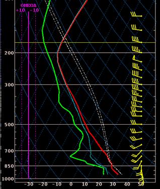
Forecast sounding valid 2100 UTC at the red dot
|
|
2100 UTC forecast sounding at the location of the red dot along the ND/SD border on the earlier maps. A few important details about the sounding: CAPE=3239 J/kg, PW=.93”, LCL=745mb, Mean RH=38%, Mean LRH=30% |
|
A) 850 hPa-300 hPa |
|
B) 850 hPa-200 hPa |
|
C) 800 hPa-200 hPa |
|
Using the sounding on the right (where the red dot was located), which of the following would not necessarily point you towards using the revised vector method to predict MCS movement across South Dakota? |
|
A) The high CAPE of 3239 J/kg |
|
B) The relatively strong unidirectional mean winds (approximately 40 kts) |
|
C) The low mean relative humidity and low relative humidity of the subcloud layer |
|
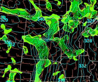
2100 UTC boundary layer winds, moisture convergence and Θe |
|
0000 UTC boundary layer winds, moisture convergence and Θe |
|
The model initialization may also not have the some important boundaries very well defined. Note the lack of low level convergence with the front in western North and South Dakota. |
|
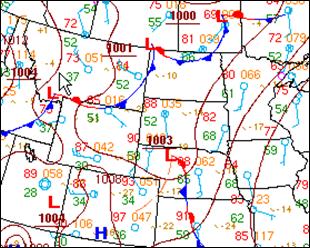
A NAM 2100 UTC MSLP and 1000-500 hPa thickness forecast valid at 2100 UTC and an HPC MSLP analysis verifying at the same time as shown below. The red and blue dot are location where NAM model soundings were secured to aid in the forecast |
|
NAM MSLP forecast valid at 2100 UTC, the red and blue dot locations is where model sounding below were chosen. |
|
2100 UTC HPC surface map
|
|
In what way might the low level convergence near the front change the stability from what the model is forecasting. |
|
B) CAPE forecasts might be higher and CIN might be lower in southeastern Montana, northeastern Wyoming and western South Dakota than predicted by the NAM. |
|
A) CAPE forecasts might be lower and CIN might be lower in southeastern Montana, northeastern Wyoming and western South Dakota than predicted by the NAM. |