|
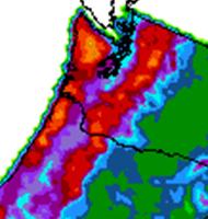
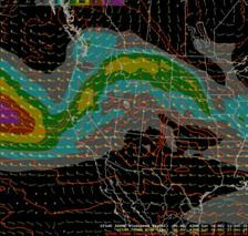
24-h analog ensemble QPF-90th percentile (upper decile) (in) product valid 1200 UTC 7 Nov. 2006. |
|
The Hamill and Whitaker reforecast method also can be used to provide a guidance product that tells the forecaster the precipitation amount that was only exceeded in 10 percent of the cases identified for that particular day. The graphic below left is such a product for the 24 hrs ending at 1200 UTC 7 Nov. 2006. |
|
The greater than 3 SD and 5 SD departure from normal for PW and 850-hPa moisture flux predicted by the SREF ensemble mean suggests that this event will at least equal the 24-h QPF from upper 10% of the reforecast project analogs suggesting a heavier rainfall maximum over the Olympic Mountains and coastal ranges of northwest Oregon than predicted by the NAM or GFS. |
|
One downside of the technique is that the forecasts are predicated on a low resolution ensemble forecast system which may not be a skillful as the SREFS. Therefore, the high precipitation amounts on the decile product can extend over too large an area at times in the shorter time range when in reality the SREF output is suggesting that the spread is quite small and that the heavy amounts will be confined to those areas with strong moisture transport and strong orographic lifting. |
|
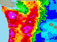
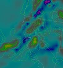
24-h accumulated precipitation (4 km grid) valid 1200 UTC 7 Nov. 2006. |
|
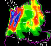
24-h accumulated precipitation (32 km grid) valid 1200 UTC 7 Nov. 2006. |
|
Two different precipitation analyses are shown for the event, one a mapped to 32-km, the other to 4-km. During this period, Lee’s Camp in Oregon received 14.3 inches and June Lake in Washington received over 15. Record flooding was reported on 10 rivers and 16 counties were declared to be in a state of emergency by the governor or Washington. The standardized anomalies correctly identified the potential for a rare event. For a summary of the effects of the event on the Oregon and Washington see http://www.ocs.orst.edu/page_links/whats_new/november_flooding.html. |
|
Leeside cool season spillover events |
|
There is usually a significant “rain shadow” to the lee of major mountain ranges like the Sierra Nevada range of California and the Cascade range of Oregon and Washington. However, there are cases when the “shadowing” effect is minimized. Wallmann and Milne (2007) (henceforth WM) note that there are a lot of misconceptions about when the “rains shadow effect” will be strong or weak. They site the following taken from NWS Forecast discussions. “South winds across the Sierra Nevada will limit the rain-shadow effect and result in more precipitation for Reno,” “moisture depth will be sufficient for precipitation to spill over into western Nevada,”strong southwest winds will result in a strong rainshadow effect.” None of these “rules of thumb” works particularly well since they are not based on scientific understanding of the blocking and the effect it has on the “rain shadow.” This section which will attempt to provide a better understanding of the “rain shadow” draws heavily on the work done by Wallmann and Milne (2007) and on Wallman’s 2007 presentation at HPC. |
|
Research by Colle (2004) identified a number of factors that affect the distribution of orographic precipitation. He noted that the distribution was “highly dependent” on how the terrain-induced gravity wave modifies the circulation aloft. His research suggests that the amount of precipitation that “spills over” the mountain crest is a function of stability, mountain height and width, wind shear, and freezing level.
Colle’s research indicates that the amount of precipitation that spills over the mountains increases and the stability decreases and as the wind speed increases and also indicates that a higher proportion of the condensate fall on the windward slopes when the freezing level is high versus when it is low if all other factors are equal. When the freezing level is high, most of the condensate is in the form a rain which falls quicker which positions the rainfall farther upstream from the mountain crest than when the freezing level is low. |
|
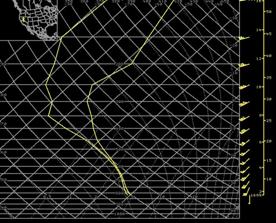
When trying to decide how much precipitation will slop over, probably the most important factor is the stability. When the air mass is stable, blocking occurs even when there is strong winds into the terrain. Also, strong southwesterly flow towards the mountains can lead to the development of a southerly barrier jet. Not much precipitation makes it to the lee side except for brief showers. WM offered the following sounding as typical of a blocking case and accompanying radar image. They note that the stable isothermal layer from 750-hPa to 675-hPa and less unstable layer above it is very indicative of cases with strong subsidence resulting in a enhanced “rain shadow”. |
|
A similar stable layer near the crest level has been noted in downsloping wind events to the lee of mountains (Colle and Mass 1998). |

|
0600 UTC 31 Dec. 2004 KREV sounding |
|
0600 UTC 31 Dec. 2004 radar reflectivity. Red lines are Nevada state line. |
|
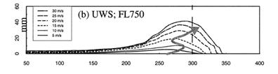
The WM paper also offers the following sounding as an example of an unstable one where there was significant spillover of precipitation to the lee of the mountains. Note that it is only barely unstable in the classical sense in the layer between the two lines. They note that there will be some spillover for weakly stable events but that they will not have the precipitation extend as far downstream as the unstable cases. For weakly stable cases, how far it extends downstream from the mountains crest is dependent on the wind. The figure below shows the simulation of rainfall with respect to the crest of a mountain for different wind speeds when the static stability is weak. Note that there is little spillover with weak winds with the maximum rainfall on the lower slopes of the terrain. As wind speeds increased, the maximum shifted towards the crest and the distance the rainfall extended downstream from the crest increased. |
|
Rainfall distribution with respect to the mountains crest (vertical dashed line) for various wind speeds under weakly stable conditions. The gray line with an arrow head is the location where the maximum increase in precipitation was found as the wind was increased to the next level. (From Colle 2004). |
|
Wallmann cautions that even when the air mass is unstable there usually needs to be some kind of synoptic or mesoscale forcing to realize the instability to get precipitation to extend well east of the mountains when the winds are below 30 knots. Without forcing, precipitation east of the mountains will usually weaken and be scattered. He also for jet streaks, frontogenesis and isentropic lift to assess the synoptic and mesoscale forcing and cautions against using Q-vectors as they lack the mesoscale resolution needed to distinguish the scale of the lifting. My own feeling is that looking at the isentropic lift to the lee of the mountains often has the same problem. However, Wallmann that in a moist, weakling stable airmass, its presence can help nudge the “rain shadow” downstream from the mountains. |
|
GFS forecast of 700-hPA frontogenesis (shaded, warm colors are frontogenetic) and 850-500-hPa moisture convergence (dashed show convergence) v.t. 1800 UTC 31 Dec. 2005. |
|
GFS forecast of 250-hPa isotachs (color fill), 700-hPa winds and temperatures v.t. 1800 UTC 31 Dec. 2005. (Images from Wallmann) |
|
A strong jet streak on the west side of the shortwave approaching the coast argues that it will remain strong as it pushes eastward and might even amplify. The entrance region of a jet streak is developing and is associated with frontogenesis and low and mid-level convergence (dashed area) and noted that by 1800 UTC the spillover would be ongoing if the model was correct. |