|
GFS model |
|
The Arakawa-Schubert (A/S) convective parameterization scheme is used in the GFS (and in the RSM members of the Short Range Ensemble Forecast System (SREF)). Details about the scheme can be found at the UCAR model matrix site (http://www.meted.ucar.edu/nwp/pcu2/avncp1.htm). There are a few things a forecaster should realize about the A/S scheme. For example, the CAP is not directly considered. However, when the scheme is activated, updrafts are entrained to the LFC which acts to reduce CAPE when dry air is present in association with a CAP. The scheme can predict elevated convection but only approximately the lowest 300-hPa of the atmosphere. The scheme is very susceptible to grid scale convective blow-ups when the airmass is very moist and unstable. The feedback associated with these blow-ups tends to produce the overdevelopment of frontal waves. The blow-ups also tend to occur later than the actual convection and over the sloping baroclinic zone. This usually leads to the grid scale bomb being north of the actually precipitation maximum. The observed maximum is usually located closer to the warm air and region of higher precipitable water than the predicted maximum which is often located over sloped isentropes associated with the frontal zone.
The GFS overpredicts total rainfall in cold and warm seasons.
|
|
The GFS model has had a resolution of about 40 km since May 2005. When using the model it is important to remember that its resolution is still not capable of resolving some mesoscale features. The resolution of the model limits the scale of the diabatic physical processes that can be are resolved and maintained by the model. For addition discussion of resolution issues see http://www.meted.ucar.edu/nwp/pcu2/avhres3.htm
In the fall of 2006 the GFS still used a rather simple cloud and grid scale precipitation parameterization scheme (Zhao and Carr 1997). This scheme predicts cloud liquid and ice based on relative humidity and temperature at each layer. It allows clouds to be advected but does not allow hydrometeors to advect as they fall. Therefore in cases where strong warm advection is taking place, the model may be too slow to spread precipitation north or northeast with the flow. However, the GFS has a high bias for lighter rainfall amounts that may somewhat offset the effects of the lack of horizontal advection of the hydrometeor. A simple scheme usually will do a relatively good job of predicting the precipitation when large scale synoptic forcing is present providing that the model has a decent mass (pressure, temperature and height) and wind field forecasts. A more complete discussion of the simple scheme that is/was used in the fall of 2007 is available at http://www.meted.ucar.edu/nwp/pcu2/avncpmp1.htm
The GFS is expected to move to the Ferrier scheme in 2007, the same scheme used in the nam/wrf. However, currently it still uses a simple cloud scheme. All the precipitation falls in one time step so the effects of dry advection on hydrometeors is ignored. Dry layers near the surface may reach saturation too soon. Also, behind a surface low where cold advection is occurring, the GFS often forecasts a large area of light precipitation and overpredicts light precipitation as there is no efficient mechanism to allow the hydrometeors to evaporate before reaching the ground.
|
|
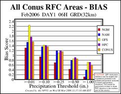
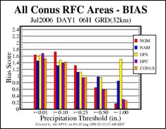
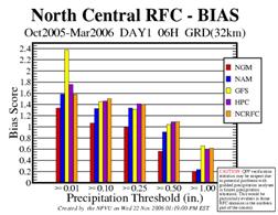
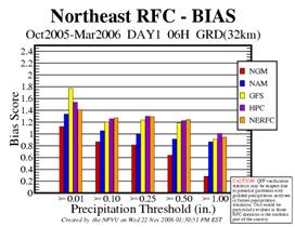
While the two graphs above only show the bias for one winter and summer month, they are very representative of the differences in bias characteristics of the GFS between the cold and warm seasons. The GFS bias for 0.01 inches or more over the U.S. during the period from November through March varied between 1.8 and 2.2 for all 6 hour periods. The bias during the warm season for 0.01 inches or more was generally around 1.6. |

|
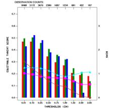
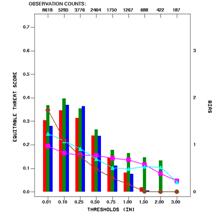
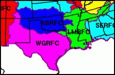
There are also considerable regional differences in the GFS performance. During the cold season when you combine 6-hourly QPF during the day 1 forecast, the GFS has a high bias for even the high precipitation threshold |
|
The 24 hr bias for heavier amounts tends to be high during the months with the greatest moisture and instability. The high bias for the 2.00 inch greater amounts probably is related to the grid scale feedback problems discussed earlier. The bias over the CONUS for the precipitation thresholds greater than 0.50, 1.00 and 2.00 is greater for the day 1 period (12-36 hr forecast) than for the day 2 or day 3 forecast with the bias for these thresholds decreasing as the lead time of the forecast increases. |
|
In winter, the GFS tends to overpredict the areal extent of 06 hourly QPF for most thresholds across MBRFC area and to a lesser extent the upper Mississippi Valley regions. This often results the in the model overpredicting the 24 hour precipitation across these regions. |
|
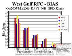
Farther south (see above), the GFS underpredicts the 0.50 inch or greater amounts during the combined 6 hourly periods of the day 1 forecast and significantly underpredicted the 1.00 inch or greater amounts during the Jan-Feb period especially at the longer time ranges. |
|
A 3-month verification over the Gulf coast region suggests that GFS and NAM/WRF bias for heavier precipitation decreases with time with the bias being quite low in day 2 and 3 time ranges. A similar bias was noted during the spring period. |
|
Day 1 bias for 1.00” or greater amounts |
|
Day 3 bias for 1.00” or greater amounts |


|
60-84 hr scores over Gulf Coast for Region for 3 month period Sept-Nov |
|
12-36 hr scores over Gulf Coast Region 3 month verification Sept-Nov |
|
The high bias for lighter amounts shows up clearly during the cold season over the northeast. This can lead to problems when trying to predict snowfall amounts as light precipitation during several 6-hourly periods can lead to 24-h totals of over 0.25 or greater amounts. However, some of the problems may also be due |
|
to problems gauges have in catching snowflakes which often causes an liquid equivalent amounts to be questionable and probably lower than they ought to be. |